§3 Classification
- Classification
- Linear Regression
- Logistic Regression
- Discriminant Analysis
- Bayes theorem for classification
- Classify to the highest density
- Why discriminant analysis?
- Linear Discriminant Analysis when p=1p = 1p=1
- Linear Discriminant Analysis when p>1p > 1p>1
- From δk(x)\delta_{k}(x)δk(x) to probabilities
- Types of errors
- Other forms of Discriminant Analysis
- Logistic Regression versus LDA
- Summary
Classification
- Qualitative variables take values in an unordered set .
- Given a feature vector and a qualitative response taking values in the set , the classification task is to build a function that takes as input the feature vector and predicts its value for ; i.e. .
- Often we are more interested in estimating the probabilities that belongs to each category in .
Linear Regression
-
Suppose for the Default classification task that we code
Can we simply perform a linear regression of on and classify as Yes if ?
- In this case of a binary outcome, linear regression does a good job as a classifier, and is equivalent to linear discriminant analysis which we discuss later.
- Since in the population , we might think that regression is perfect for this task.
- However, linear regression might produce probabilities less than zero or bigger than one. Logistic regression is more appropriate.
-
Now suppose we have a response variable with three possible values. A patient presents at the emergency room, and we must classify them according to their symptoms.
This coding suggests an ordering, and in fact implies that the difference between stroke and drug overdose is the same as between drug overdose and epileptic seizure.
Linear regression is not appropriate here.
Multiclass Logistic Regression or Discriminant Analysis are more appropriate.
Logistic Regression
-
Let's write for short and consider using balance to predict default. Logistic regression uses the form
( is a mathematical constant [Euler's number.])
It is easy to see that no matter what values or take, will have values between 0 and 1.
A bit of rcarrangcment gives
This monotone transformation is called the odds** or logit transformation of .
-
Logistic regression ensures that our estimate for lies
between 0 and 1.
Maximum Likelihood
-
We use maximum likelihood to estimate the parameters.
This likelihood gives the probability of the observed zeros and ones in the data. We pick and to maximize the likelihood of the observed data.
Most statistical packages can fit linear logistic regression models by maximum likelihood. In
Rwe use theglmfunction.
Confounding
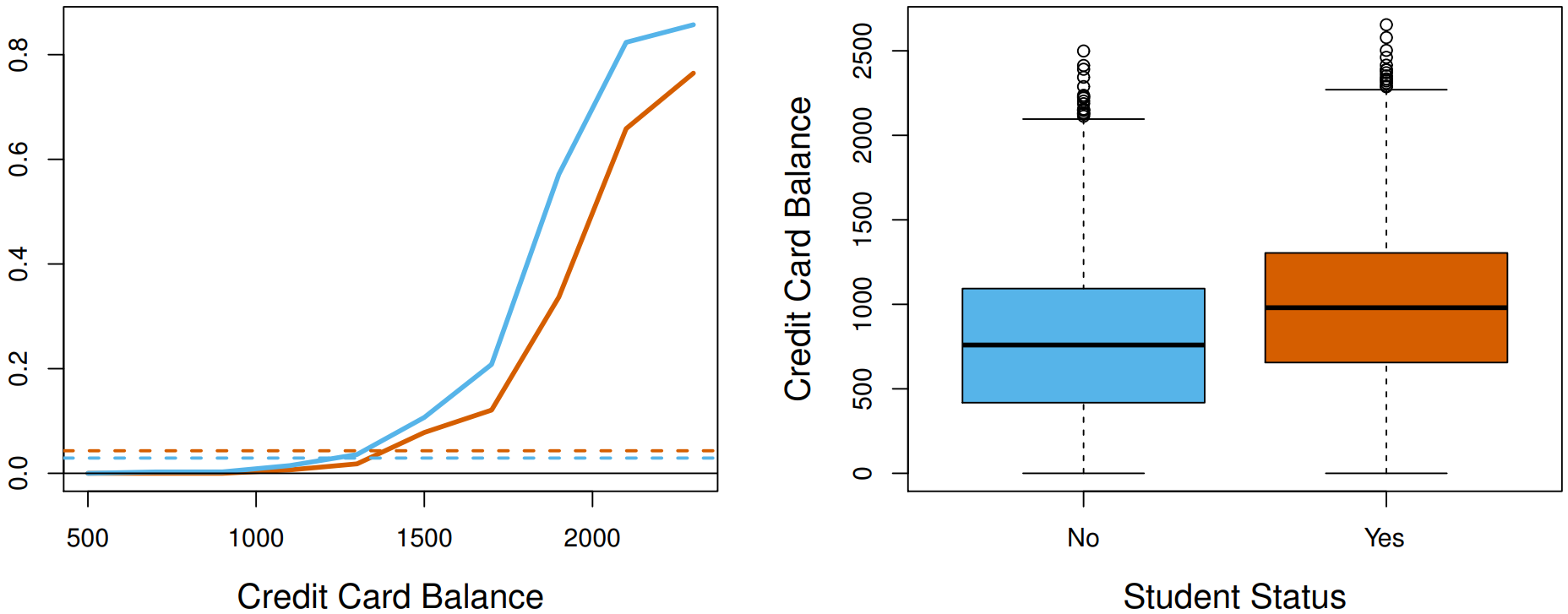
- Students tend to have higher balances than non-students, so their marginal default rate is higher than for non-students.
- But for each level of balance, students default less than non-students.
- Multiple logistic regression can tease this out.
Case-control sampling and logistic regression
-
In South African data, there are 160 cases, 302 controls are cases. Yet the prevalence of MI in this region is .
-
With case-control samples, we can estimate the regression parameters accurately (if our model is correct); the constant term is incorrect.
-
We can correct the estimated intercept by a simple transformation
-
Often cases are rare and we take them all; up to five times that number of controls is sufficient.
Diminishing returns in unbalanced binary data
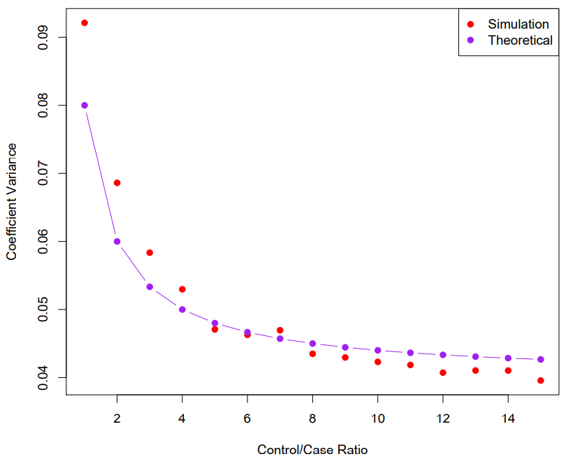
- Sampling more controls than cases reduces the variance of the parameter estimates. But after a ratio of about 5 to 1 the variance re- duction flattens out.
Logistic regression with more than two classes
-
So far we have discussed logistic regression with two classes. It is easily generalized to more than two classes. One version (used in the R package
glmnet) has the symmetric formHere there is a linear function for each class.
(Some cancellation is possible, and only linear functions are needed as in 2-class logistic regression.)Multiclass logistic regression is also referred to as multinomial regression.
Discriminant Analysis
- Here the approach is to model the distribution of in each of the classes separately, and then use Bayes theorem to flip things around and obtain .
- When we use normal (Gaussian) distributions for each class, this leads to linear or quadratic discriminant analysis.
- However, this approach is quite general, and other distributions can be used as well. We will focus on normal distributions.
Bayes theorem for classification
-
Thomas Bayes was a famous mathematician whose name represents a big subfield of statistical and probabilistic modeling. Here we focus on a simple result, known as Bayes theorem:
One writes this slightly differently for discriminant analysis:
where
- is the density for in class . Here we will use normal densities for these, separately in each class.
- is the marginal or prior probability for class .
Classify to the highest density
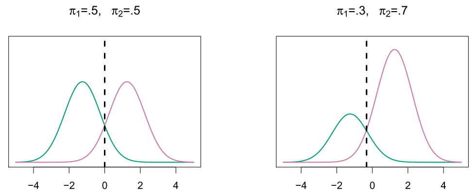
- We classify a new point according to which density is highest.
- When the priors are different, we take them into account as well, and compare . On the right, we favor the pink class - the decision boundary has shifted to the left.
Why discriminant analysis?
- When the classes are well-separated, the parameter estimates for the logistic regression model are surprisingly unstable. Linear discriminant analysis does not suffer from this problem.
- If is small and the distribution of the predictors is approximately normal in each of the classes, the linear discriminant model is again more stable than the logistic regression model.
- Linear discriminant analysis is popular when we have more than two response classes, because it also provides low-dimensional views of the data.
Linear Discriminant Analysis when
-
The Gaussian density has the form
Here is the mean, and the variance (in class ). We will assume that all the are the same.
Plugging this into Bayes formula, we get a rather complex expression for :
Happily, there are simplifications and cancellations.
Discriminant functions
-
To classify at the value , we need to see which of the is largest. Taking logs, and discarding terms that do not depend on , we see that this is equivalent to assigning to the class with the largest discriminant score:
Note that is a linear function of .
If there are classes and , then one can see that the decision boundary is at
Typically we don’t know these parameters; we just have the training data. In that case we simply estimate the parameters and plug them into the rule.
Estimating the parameters
where is the usual formula for the estimated variance in the th class.
Linear Discriminant Analysis when
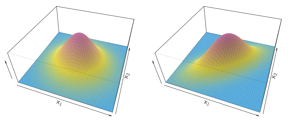
-
Density:
-
Discriminant function:
Despite its complex form, is a linear function.
Illustration: and classes
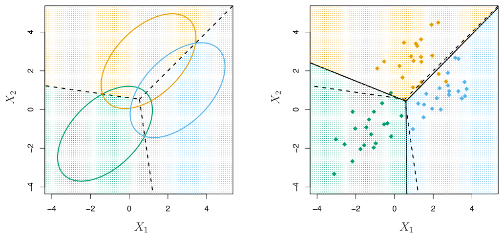
Here .
- The dashed lines are known as the Bayes decision boundaries. Were they known, they would yield the fewest misclassification errors, among all possible classifiers.
From to probabilities
-
Once we have estimates , we can turn these into estimates for class probabilities:
So classifying to the largest amounts to classifying to the class for which is largest.
When , we classify to class 2 if else to class 1.
Types of errors
-
False positive rate: The fraction of negative examples that are classified as positive.
-
False negative rate: The fraction of positive examples that are classified as negative.
-
We produced this table by classifying to class Yes if
We can change the two error rates by changing the threshold from to some other value in :
and vary threshold.
Varying the threshold
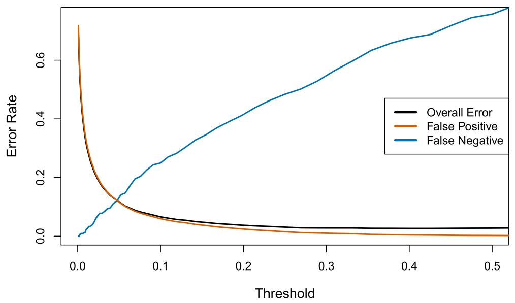
- In order to reduce the false negative rate, we may want to reduce the threshold to or less.
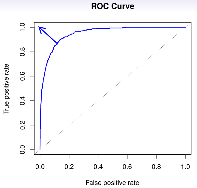
-
The ROC plot displays both simultaneously.
Sometimes we use the AUC or area under the curve to summarize the overall performance. Higher AUC is good.
Other forms of Discriminant Analysis
When are Gaussian densities, with the same covariance matrix in each class, this leads to linear discriminant analysis. By altering the forms for , we get different classifiers.
- With Gaussians but different in each class, we get quadratic discriminant analysis.
- With (conditional independence model) in each class we get naïve Bayes. For Gaussian this means the are diagonal.
- Many other forms, by proposing specific density models for , including nonparametric approaches.
Quadratic Discriminant Analysis
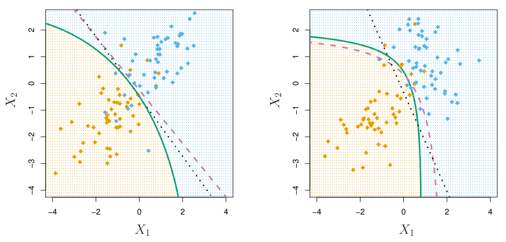
Because the are different, the quadratic terms matter.
Naïve Bayes
-
Assumes features are independent in each class.
Useful when is large, and so multivariate methods like QDA and even LDA break down.
-
Gaussian naïve Bayes assumes each is diagonal:
-
can use for mixed feature vectors (qualitative and quantitative). If is qualitative, replace with probability mass function (histogram) over discrete categories.
-
-
Despite strong assumptions, naive Bayes often produces good classification results.
Logistic Regression versus LDA
-
For a two-class problem, one can show that for LDA
So it has the same form as logistic regression.
The difference is in how the parameters are estimated.
- Logistic regression uses the conditional likelihood based on (known as discriminative learning).
- LDA uses the full likelihood based on (known as generative learning).
- Despite these differences, in practice the results are often very similar.
-
Footnote: logistic regression can also fit quadratic boundaries like QDA, by explicitly including quadratic terms in the model.
Summary
- Logistic regression is very popular for classification, especially when .
- LDA is useful when is small, or the classes are well separated, and Gaussian assumptions are reasonable. Also when .
- Naïve Bayes is useful when is very large.
— Jul 15, 2022

§3 Classification by Lu Meng is licensed under a Creative Commons Attribution-NonCommercial-ShareAlike 4.0 International License. Permissions beyond the scope of this license may be available at About.
Made with ❤ at Earth.