Simon's Algorithm

Simon’s Algorithm was first proposed by Daniel Simon in 1994. It was the first quantum algorithm that was exponentially faster than the best classical algorithm and was also an inspiration for Shor’s Algorithm.

Problem Description

Goal:

We are given a hidden function $f:\{0,1\}^n\to\{0,1\}^n$, such that $f(x)=f(y)$ if and only if $y=x$ or $y=x \oplus s$ for a secret string $s \in \{0,1\}^n$. Our goal is to find $s$.

Remarks:

• If $s=0^n$, then $f$ is one-to-one. If $s \ne 0^n$, then $f$ is two-to-one. Both cases are identifiable by Simon’s Algorithm. However, for illustration, we may assume $s \ne 0^n$ in later parts.

An example with $n=4, s=1001$:

It can be easily checked that this $f$ is a two-to-one function since exactly two different inputs are mapped to a unique output.

Solutions

Classic Solution:

If we can find $x$ and $y$ such that $x \ne y$ and $f(x)=f(y)$, then we can obtain $s=x \oplus y$. Therefore, the question now becomes how many different inputs do we have to try in order to find two inputs with the same output?

We have $2^n$ different inputs, and half of them ($2^{n-1}$ inputs) produce unique outputs.

• Worst case: We need to try $2^{n-1}+1$ inputs $\longrightarrow$ $\Theta(2^n)=\mathcal{O}(2^n)$ complexity
• Average case: We need to try approximately $2^{n/2}$ inputs (see birthday problem) $\longrightarrow$ $\Theta(2^{n/2})=\mathcal{O}(2^n)$ complexity

In fact, we can show that all classic solutions have at least $\Omega(2^{n/2})$ query complexity.

Quantum Solution:

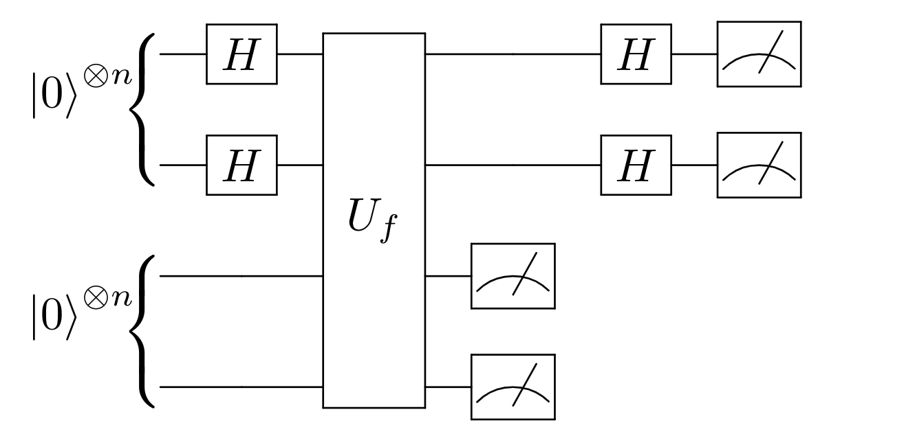
1. We initialize $2$ quantum systems $A$ and $B$ with $n$ qubits each in the state $\ket{0}$.

2. Pass each of the $n$ qubits in $A$ through a Hadamard gate.

3. Pass $A$ and $B$ through the oracle $U_f:\ket{x},\ket{y}\to\ket{x},\ket{y\oplus f(x)}$.

4. Measure $B$ on the computational basis.

5. Pass each of the $n$ qubits in $A$ through a Hadamard gate again.

6. Measure $A$ on the computational basis and record the outcome string $z_i$.

7. Repeat procedure 1-6 until we have $n-1$ linearly independent $z_i$’s.

   Then $s$ can be solved by equations:

   $$\left\{\begin{array}{c}s \cdot z_{1}=0 \mod 2 \\ s \cdot z_{2}=0 \mod 2 \\ \vdots \\ s \cdot z_{n-1}=0 \mod 2 \end{array}\right.$$

Remarks:

• The probability that $z_i$’s are not linearly independent is at most $0.711212$ (proof omitted), so we only need to repeat procedure 1-6 for $\mathcal{O}(n)$ times to satisfy the independence condition. Each time, we only query $U_f$ once. Therefore, the query complexity of Simon’s Algorithm is $\mathcal{O}(n)$, which is exponentially faster than classic algorithms.
• Although this is a system of $n-1$ linear equations in $n$ unknowns, we can still solve for a unique non-zero solution $s$. (Recall our assumption that $s \ne 0^n$)
• A detailed proof of the correctness of Simon’s Algorithm is omitted here, as we will put emphasis on how to use code to implement this quantum algorithm. However, more details can be found in References.

Implementation

Quantum Implementation:

To illustrate how to implement the quantum circuit, we use the example $f$ given in the above table.

To design a $U_f$ based on $f$:

• We notice that $f(0000)=f(1001)$. This implies we may use $x_0$ and $x_3$ to control the same $y_i$ so that the output remains unchanged for two $x$’s differing by $s=1001$.
• Since only the two-to-one mapping relations are essential, while the specific numeric numbers allocated to $f(x)$ are not. We may design the remaining part of $U_f$ through trials and errors.

The final $U_f$ is

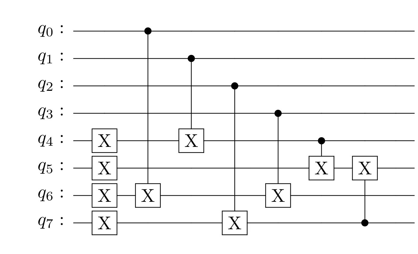
The code of this oracle is in Appendix(1.1)

With $U_f$, the full quantum circuit of Simon’s Algorithm for the example $f$ is

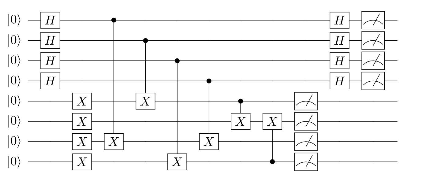
The code of this algorithm is in Appendix(1.2)

Experimental Results:

To test the performance of our implementation, we run the quantum circuit on the Quantum Leaf CloudBaiduSim2Water simulator. The server simulates the code for 1024 times and provides the histogram of raw outputs.

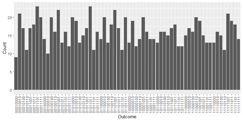
The raw outcomes are in Appendix(1.3)

However, we are only interested in the last $4$ bits measured on system $A$. After performing some data cleansing, we can obtain the desired histogram.

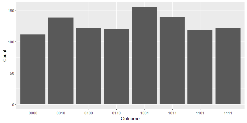
The transformed outcomes are in Appendix(1.4)

Notice that we obtain more than needed data in this simulation. So, we may randomly choose $n-1=3$ linearly independent outcomes for further post-processing. Assume the obtained outcomes are $\{0010,0100,1001\}$. We can solve for $s$ with the equation

$$\left[\begin{array}{llll}0 & 0 & 1 & 0 \\ 0 & 1 & 0 & 0 \\ 1 & 0 & 0 & 1 \\ 0 & 0 & 0 & 0\end{array}\right]\left[\begin{array}{l}s_{1} \\ s_{2} \\ s_{3} \\ s_{4}\end{array}\right]=\left[\begin{array}{l}0 \\ 0 \\ 0 \\ 0\end{array}\right]$$

where $s=\overline{s_1 s_2 s_3 s_4}$. After Gaussian elimination, the augmented matrix becomes

$$\left[\begin{array}{llll|l}1 & 0 & 0 & 1 & 0 \\ 0 & 1 & 0 & 0 & 0 \\ 0 & 0 & 1 & 0 & 0 \\ 0 & 0 & 0 & 0 & 0\end{array}\right]$$

A non-trial solution (i.e. $s \ne 0000$) to this equation is $s=1001$.

If we pick any other set of linearly independent outcomes, the result is the same. In this way, we have shown the correctness of our quantum implementation.

References

1. Johansson, N.; Larsson, JÅ. (2017). “Efficient classical simulation of the Deutsch–Jozsa and Simon’s algorithms”. Quantum Inf Process (2017). 16 (9): 233. arXiv:1508.05027. Bibcode:2017QuIP…16…233J. doi:10.1007/s11128-017-1679-7. S2CID 28670540.
2. Koiran, P.; Nesme, V.; Portier, N. (2005), “A quantum lower bound for the query complexity of Simon’s Problem”, Proc. ICALP, 3580: 1287–1298, arXiv:quant-ph/0501060, Bibcode:2005quant.ph…1060K, retrieved 2011-06-06
3. Qiskit. Simon’s Algorithm. Retrieved from https://qiskit.org/textbook/ch-algorithms/simon.html.
4. Simon, Daniel R. (1997-10-01). “On the Power of Quantum Computation”. SIAM Journal on Computing. 26 (5): 1474–1483. doi:10.1137/S0097539796298637. ISSN 0097-5397.

Technical Instructions

How to use Quantum Leaf?

1. Register and login https://quantum-hub.baidu.com/.
2. Click QComposer on the side panel.
3. Copy and paste codes into the code space on the left.
4. Select a Quantum End in the upper right corner and click Run.
5. After execution, results will be shown at the bottom.

Appendix

1.1 Code of $U_f$ for Simon’s Algorithm

OPENQASM 2.0;
include "qelib1.inc";
qreg q[8];
creg c[8];
//
x q[4];
x q[5];
x q[6];
x q[7];
//
cx q[0], q[6];
//
cx q[1], q[4];
//
cx q[2], q[7];
//
cx q[3], q[6];
//
cx q[4], q[5];
//
cx q[7], q[5];

1.2 Code of Simon’s Algorithm

OPENQASM 2.0;
include "qelib1.inc";
qreg q[8];
creg c[8];
//
h q[0];
h q[1];
h q[2];
h q[3];
//
x q[4];
x q[5];
x q[6];
x q[7];
//
cx q[0], q[6];
//
cx q[1], q[4];
//
cx q[2], q[7];
//
cx q[3], q[6];
//
cx q[4], q[5];
//
cx q[7], q[5];
//
//
h q[0];
h q[1];
h q[2];

h q[3];
//
measure q[4] -> c[4];
measure q[5] -> c[5];
measure q[6] -> c[6];
measure q[7] -> c[7];
measure q[0] -> c[0];
measure q[1] -> c[1];
measure q[2] -> c[2];
measure q[3] -> c[3];

1.3 Raw outcomes of Simon’s Algorithm

{
    "00010000": 9,
    "00010010": 21,
    "00010100": 17,
    "00010110": 11,
    "00011001": 17,
    "00011011": 18,
    "00011101": 23,
    "00011111": 20,
    "00100000": 14,
    "00100010": 10,
    "00100100": 20,
    "00100110": 16,
    "00101001": 22,
    "00101011": 13,
    "00101101": 16,
    "00101111": 12,
    "01010000": 20,
    "01010010": 19,
    "01010100": 13,
    "01010110": 15,
    "01011001": 17,
    "01011011": 23,
    "01011101": 11,
    "01011111": 16,
    "01100000": 14,
    "01100010": 20,
    "01100100": 13,
    "01100110": 18,
    "01101001": 22,
    "01101011": 17,
    "01101101": 11,
    "01101111": 20,
    "10000000": 13,
    "10000010": 19,
    "10000100": 12,
    "10000110": 14,
    "10001001": 20,
    "10001011": 16,
    "10001101": 14,
    "10001111": 14,
    "10110000": 13,
    "10110010": 16,
    "10110100": 16,
    "10110110": 15,
    "10111001": 17,
    "10111011": 18,
    "10111101": 12,
    "10111111": 12,
    "11000000": 15,
    "11000010": 17,
    "11000100": 16,
    "11000110": 20,
    "11001001": 19,
    "11001011": 15,
    "11001101": 13,
    "11001111": 13,
    "11110000": 13,
    "11110010": 16,
    "11110100": 15,
    "11110110": 11,
    "11111001": 21,
    "11111011": 19,
    "11111101": 18,
    "11111111": 14
}

1.4 Transformed outcomes of Simon’s Algorithm

{
    "0000": 111,
    "0010": 138,
    "0100": 122,
    "0110": 120,
    "1001": 155,
    "1011": 139,
    "1101": 118,
    "1111": 121,
}

— Oct 30, 2021

Simon's Algorithm by Lu Meng is licensed under a Creative Commons Attribution-NonCommercial-ShareAlike 4.0 International License. Permissions beyond the scope of this license may be available at About.